
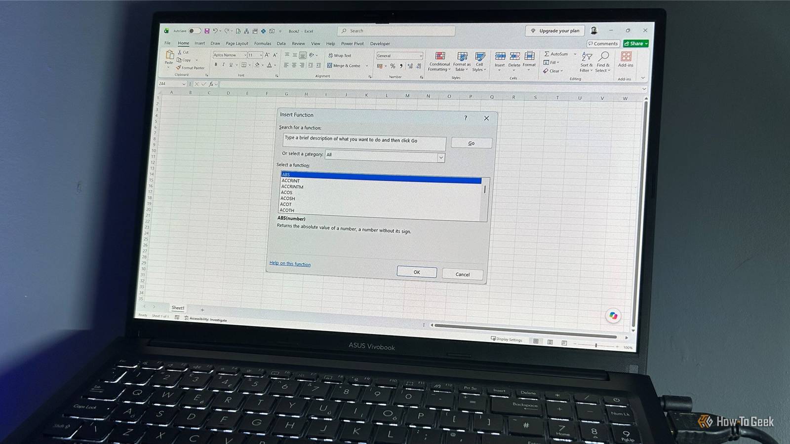
Excel has hundreds of functions, and I certainly don't know what all of them do.But every now and then, I find one that makes me wonder why I'd never come across it before.Here are seven that caught me by surprise.
I've used regular cell references in the examples rather than Excel tables, so the formulas are easier to follow.GESTEP: Check whether a number has reached a threshold A tiny function for a common question GESTEP checks whether a number has reached a specified threshold, returning 1 if it has and 0 if it hasn't.Say you're tracking your daily steps and want Excel to flag the days when you reached your 10,000-step goal: =GESTEP(B2,$E$2) where B2 contains the number of steps, and E2 contains the target.
It's essentially the same result as =IF(B2>=$E$2,1,0), but GESTEP makes the purpose immediately obvious: you're testing whether the number has reached your target.That makes it useful for tracking everyday things, from steps and calories to savings and points.Because the result is numeric, you can also use it directly in further calculations.
CONVERT: Switch between measurements Stop hunting for conversion factors CONVERT switches a value from one measurement unit to another.Suppose you're looking at a piece of furniture online and its dimensions are given in inches, but you've measured the space in centimeters.You could enter this: =CONVERT(B2,$B$1,$C$1) where B2 contains the value in inches, B1 contains the starting unit, and C1 contains the target unit.
Excel handles the conversion for you, and because the unit codes are in cells, you can change them without rewriting the formula.CONVERT supports units for distance, weight, temperature, time, and several other measurements.It's particularly handy for DIY projects, recipes, travel, or any situation where you need to switch between units.
ROMAN: Generate Roman numerals automatically Even Excel can get a little theatrical ROMAN converts ordinary numbers into Roman numerals.Imagine you're creating a document or presentation outline and want a list numbered I, II, III, and so on instead of 1, 2, 3.The formula is straightforward: =ROMAN(SEQUENCE(10)) SEQUENCE generates the numbers, while ROMAN converts them, giving you a spilled list of Roman numerals automatically.
You could use the same trick for sections, stages, or any other numbered list where you want something a little more distinctive.You might not use ROMAN every day, but combining it with SEQUENCE turns an obscure function into a surprisingly neat little trick.REPT: Create mini charts inside cells Who says a chart needs its own chart object? REPT repeats a piece of text as many times as you specify.
Yes, this sounds mundane, but imagine you've made a simple spreadsheet to track your progress toward a savings goal, and you want each row to show a visual indicator without inserting a chart.If B2 contains the target amount and C2 contains the amount you've saved so far, you can use this formula in D2: =REPT("",MIN(10,ROUND(C2/B2*10,0)))&REPT("♡",MAX(0,10-ROUND(C2/B2*10,0))) This calculates what percentage of the target you've reached, caps it at 100%, and turns it into a row of 10 hearts, using filled hearts for the completed portion and empty hearts for the rest.You can use the same idea for habit trackers, ratings, or other personal projects where a simple indicator makes things easier to visualize.
Because the result lives inside a cell, it stays alongside the data and doesn't need a separate chart object.Change the underlying numbers and the indicator changes with them.Conditional formatting data bars are another way to visualize numbers, but REPT lets you choose the character you want to repeat.
ABS: See how far a number is from another Sometimes the direction of the difference doesn't matter ABS returns the absolute value of a number, removing its negative sign.Suppose you're cutting several pieces for a DIY project, and each one has a target measurement with a little room for error.Here's what you can enter: =ABS(C2-B2)<=D2 This calculates the difference between the measurement in C2 and the target in B2, removes its direction, and checks whether that difference is within the tolerance in D2.
If it is, the formula returns TRUE (which checks the box), and if it isn't, it returns FALSE (which leaves the box unchecked).This is useful whenever you care about the size of a difference rather than whether you're above or below the target.The same approach works for cooking, fitness goals, or any other situation with an acceptable margin of error.
You could also use AND to test whether a value falls between two limits, but ABS lets you calculate the size of the difference from the target first, which can be useful if you want to use that difference in a further calculation.TRUNC: Find how many complete things you can have Excel can't give you part of a box TRUNC removes the fractional part of a number without rounding it.Say you have $47 to spend, and each item costs $6.
A standard division gives you 7.83 items, but you can only buy seven.Instead, use TRUNC: =TRUNC(A3/B3) TRUNC returns 7, giving you the number of complete items you can actually have.The same idea works for complete boxes, whole weeks, full teams, or any other quantity where the fraction isn't useful.
Unlike FLOOR and CEILING, which round to a specified multiple, TRUNC simply removes the fractional portion.Excel has several other rounding functions too, including ROUNDUP, ROUNDDOWN, and INT.While some of these produce the same result for positive numbers, they behave differently with negative numbers or when you're rounding to a specific multiple.
MAXIFS: Find the highest value that meets your criteria Finding the biggest number gets more interesting when you add conditions Close MAXIFS finds the largest value in a range while applying one or more criteria.Imagine you've organized your purchases in an Excel sheet with columns for Date, Amount, Store, and Category.Now you want to find the largest amount you've spent on the category typed into F2: =MAXIFS(B2:B11,D2:D11,F2) where B2:B11 contains the values to evaluate, D2:D11 contains the criteria range, and F2 contains the category you're looking for.
You can add another condition to ask a more specific question: What's the largest purchase you've made in a particular category (F2) at a particular store (G2)? =MAXIFS(B2:B11,D2:D11,F2,C2:C11,G2) This method lets you change the criteria cells to investigate different combinations without filtering your data.And if you need to find the smallest value that meets the same kind of conditions, MINIFS works in exactly the same way.Got a problem? There's probably an Excel function for that You don't need to memorize every Excel function.
What matters more is knowing that Excel probably has a function for the oddly specific problem you've just encountered.The next time you're about to build a complicated workaround, it might be worth searching the function list first.You may find that Excel has already done the hard work for you.
Read More