Manually re-sorting your Excel tables every time a score changes is a waste of time.The RANK.EQ function automates leaderboards by assigning positions instantly.Whether you're tracking sales or race times, here's how to keep your data dynamic and accurate.
Previously, RANK was Excel's only ranking function.However, in 2010, Microsoft introduced RANK.EQ (identical to the old RANK) and RANK.AVG (a new option that returns the average rank for ties).In this guide, I'll use RANK.EQ, since it's the modern standard and works in exactly the same way as RANK.
How the RANK.EQ function works Understanding the syntax The RANK.EQ function identifies where a number sits relative to others in a list, providing a "live" standing that updates automatically.The function follows a straightforward syntax: =RANK.EQ(number, ref, [order]) where: number (required) is the value you want to rank.ref (required) is the range or array of numbers you're comparing the value against.
Non-numeric values (like text or blanks) are ignored.order (optional) determines the ranking direction.Use 0 (or leave it blank) for a descending rank, or 1 for an ascending rank.
If multiple values have the same rank, RANK.EQ assigns them the top rank of that group.For example, if two people tie for the highest score, they both receive a rank of 1, and the next highest score receives a rank of 3.The RANK function works best with Excel tables because they handle range expansion and structured references automatically.
However, if you use a regular cell range, lock your ref using dollar signs—such as $B$2:$B$10.To follow along as you read, download a free copy of the Excel workbook used in the examples.After you click the link, you'll find the download button in the top-right corner of your screen, and when you open the file, you can access each use case on a separate worksheet tab.
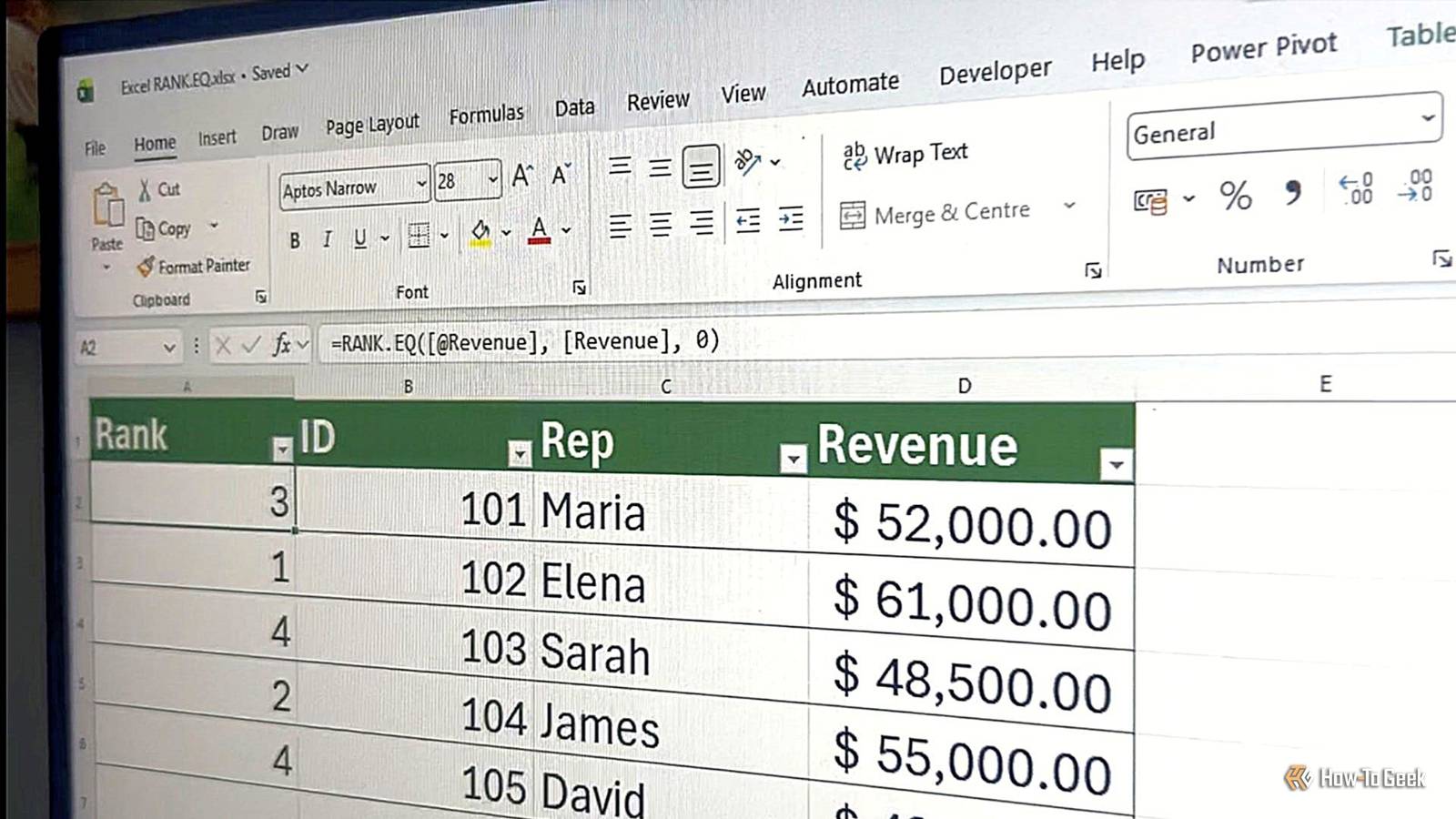
Use case 1: Building a dynamic leaderboard Rank entries without reordering rows RANK.EQ identifies top performers while keeping your data in its original order.The scenario: You have an Excel table named T_Sales.It includes an ID column representing the order in which details were signed.
You want the rank in column A so the standings are visible, but you must keep the table sorted by ID to match your physical receipts.To generate these standings, type this formula into cell A2 and press Enter: =RANK.EQ([@Revenue], [Revenue], 0) Here's how the formula works: [@Revenue] looks at the revenue for the current row.For ID 101, it sees 52000.
[Revenue] compares that value against every number in the entire column.0 ensures the person with the highest revenue (Elena) is assigned rank 1.You could leave this out for a cleaner formula.
Why not just use table sorting? It's tempting just to sort from largest to smallest using the filter arrow at the top of the Revenue column.However, as well as messing up your original ID order, it's a static fix for a dynamic problem.As soon as you add a new sale or update a revenue figure, you would need to reapply or maintain the sort.
By using RANK.EQ, you create a "set it and forget it" system.It allows you to keep your main table in its original order, and the formula expands downward to any new rows you add, meaning the rankings update instantly.Make the most of your data To make the result even more meaningful, use the rank in column A as the engine for a SORTBY formula to automatically display your data from rank 1 downward.
In a blank cell, type: =SORTBY(T_Sales, T_Sales[Rank], 1) This creates a dynamic copy of your table that stays ordered from 1 to 5.Even though your source table remains sorted by ID, this new list ensures that rank 1 always sits at the top.As soon as the data changes, this list updates automatically.
Use case 2: Ranking fastest times Handle scenarios where the lowest number wins By flipping the order argument of the RANK.EQ function, you can ensure that the smallest numbers are recognized as the "winners." The scenario: You're tracking lap times in a table named T_Results.You need to keep this table in its original order of the starting grid (StartPos), but you still want to know who currently holds the fastest lap.To rank these from fastest to slowest, type this formula into cell B2: =RANK.EQ([@Seconds], [Seconds], 1) This time, setting the order argument to 1 uses ascending ranking, ensuring the lowest time is rank 1.
Make the most of your data By placing the rank in column B, you can extract a clean podium display using the FILTER and SORT functions together in a separate cell: =SORT(FILTER(T_Results[[Rank]:[Seconds]], T_Results[Rank] <= 3), 1, 1) This creates a secondary array that pulls only the fastest three drivers.Because it's linked to the Rank column, the podium updates automatically even though your main table stays sorted by the StartPos column.Use case 3: Breaking ties using a secondary metric Use bonus points to decide the final standings RANK.EQ assigns the same rank to tied scores.
To create a unique ranking that rewards secondary performance (like bonus points), you can add COUNTIFS to your formula.This counts how many people share the same score but have a higher bonus.Subscribe to the newsletter for more Excel wins Want more practical Excel techniques, formulas, and ready-to-use workbook examples? Subscribe to the newsletter to get curated walkthroughs, tie-breaker tricks, and table-ready templates that help you automate leaderboards and rankings.
Get Updates By subscribing, you agree to receive newsletter and marketing emails, and accept our Terms of Use and Privacy Policy.You can unsubscribe anytime.The scenario: You have a table named T_League.
Three players are tied at 88 points, so you want to use their bonus points to break the tie so that every rank is unique and fair.To create a unique, merit-based ranking, type this formula into cell A2: =RANK.EQ([@Points], [Points]) + COUNTIFS([Points], [@Points], [Bonus], ">"&[@Bonus]) This formula calculates a base rank, then "pushes" tied players down based on their bonus points: RANK.EQ([@Points], [Points]) identifies the standard rank.For all three players with 88 points, this returns 2 (because Dakota is #1).
COUNTIFS(...) is the tie-breaker.It looks only at players who have exactly the same points as the current row and counts how many of them have a bonus higher than the current row.Let's take Blake (88 points, 15 bonus) as an example: RANK.EQ sees that Blake is tied for rank 2.
COUNTIFS looks at everyone with 88 points and asks, "Who has a bonus higher than Blake's 15?" Only Emerson qualifies, so the count is 1.Excel then adds that count (1) to the base rank (2).As a result, Blake is identified as rank 3.
Because this method uses standard functions, it's incredibly fast, returns a single value per row (making it ideal for Excel tables), and is easy for others to understand.These ranking techniques ensure every new entry finds its place on the leaderboard the second you type it in—meaning it's a huge win for anyone tracking live competitive data.That said, if you just need a sequential list that reacts to your data entries or deletions as they happen, combine the SEQUENCE and COUNTA functions.
Either way, the key is automation and time-saving—benefits both these Excel workflows offer.Microsoft 365 Personal OS Windows, macOS, iPhone, iPad, Android Free trial 1 month Microsoft 365 includes access to Office apps like Word, Excel, and PowerPoint on up to five devices, 1 TB of OneDrive storage, and more.$100 at Microsoft Expand Collapse
Read More