
If you've spent any time working with data in Excel, you've probably come across filtering.It's a quick way to focus on the records you need, analyze a subset of your data, and hide everything else from view.But Excel's regular filter buttons come with a few annoyances: they hide entire worksheet rows, can make the original dataset harder to see, and leave you with filters to clear when you've finished.
That's where the FILTER function comes in.It creates a separate, live list of matching records, so your original data stays visible and untouched.And with a couple of nifty little tricks, FILTER is more flexible than you might first imagine.
FILTER creates a separate, live list from your data Leave your source intact FILTER uses three arguments: =FILTER(array,include,[if_empty]) The first argument, array, is the data you want FILTER to return, whether that's a whole table, a single column, or several adjacent columns.The second, include, tells Excel which rows to include in the results.The optional third argument, if_empty, lets you specify what should appear if there are no matching records.
FILTER works particularly well when your source data is an Excel table.Instead of pointing to a fixed range such as A2:D101, you can use the table's name and structured references, so the formula automatically picks up new rows added to the source data.There's one important catch: the FILTER formula itself needs to sit outside the Excel table.
Its results spill into the cells below and beside the formula, and dynamic arrays can't spill inside a table.For this reason, make sure there's enough room for the results to spill, or Excel will return a #SPILL! error.Once that's set up, you can begin building your formula.
Start with a single condition Let one cell control the results Close I use an Excel table named GolfData to keep track of my golf scores.Next to the table, I have a small criteria area with a data validation drop-down menu in cell F2 containing the course names.When I select a course, the FILTER function returns every round I've played there.
I could hard-code the course name into the formula, but using a cell reference means I can change the criteria without editing the formula.In this case, F2 contains whatever course I've selected from the drop-down menu.Here's the formula: =FILTER(GolfData,GolfData[Course]=F2,"No rounds found") If you're building a formula with several criteria, press Alt+Enter as you type to insert a line break.
The first argument tells FILTER to return the entire GolfData table, the second checks each row in the Course column against whatever I've selected in F2, and the third specifies the text I want to return if there are no matches.The result spills into the worksheet as a separate, live list, containing only the rows that match my selected course.Change the drop-down selection, and the list changes with it.
Because FILTER creates a spilled range, I can also refer to the entire result from another formula using the spill range operator (#).For example, if my FILTER formula starts in F5, =ROWS(F5#) counts the number of records currently returned by the formula.Change the course in F2, and the count updates automatically.
Add more conditions as your needs change FILTER can check several criteria A single condition is useful, but I can make the same formula more selective without starting over.This time, I've added start and end dates in G2 and H2.Now, I can filter the results to see rounds for my selected course that fall between those two dates.
The good thing is that all I need to do is add those conditions to the existing formula: =FILTER(GolfData,(GolfData[Course]=F2) *(GolfData[Date]>=G2) *(GolfData[Date]<=H2),"No rounds found") The * symbol represents AND logic here, meaning all three conditions must be met.In other words, to be included in the result, a row has to: Match the selected course, and Be on or after the start date, and Be on or before the end date.This is one of the things I like about FILTER: I can keep extending the same basic formula as my requirements become more specific.
I don't have to create a separate filtering setup every time I want to narrow the results.Related The Beginner's Guide to Boolean Logic in Microsoft Excel Boost your Boolean boon.Posts 2 By Tony Phillips Mix and match different criteria Keep stacking conditions when you need them I can take this another step by adding a weather condition.
I've added another data validation drop-down menu in I2, containing the four weather categories in my dataset.Now I want only the rounds that match my selected course, fall within my date range, and took place in the selected weather.The formula becomes: =FILTER(GolfData,(GolfData[Course]=F2) *(GolfData[Date]>=G2) *(GolfData[Date]<=H2) *(GolfData[Weather]=I2), "No rounds found") I can change the course, dates, or weather from the criteria cells, and the spilled list updates automatically.
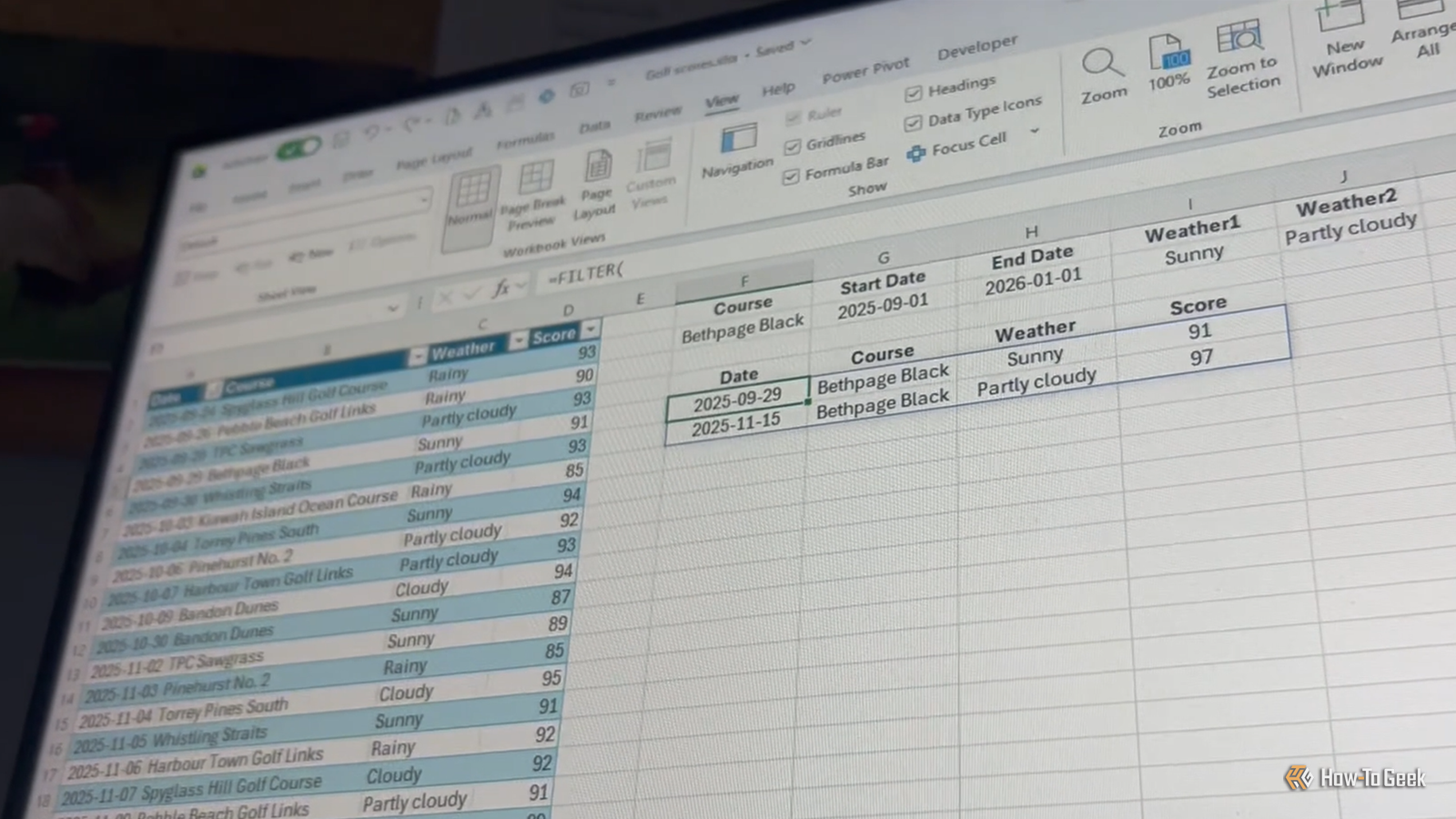
Because the formula is separate from the source data, I can also see my original dataset at the same time.Use OR when either condition will do A plus sign changes the logic So far, I've required every condition to be met.But what if I want to see rounds played in either of two types of weather? I'll keep my course and date criteria, but add a second weather drop-down menu in J2.
Now I can select, for example, "Sunny" in I2 and "Partly cloudy" in J2.Here's the formula: =FILTER(GolfData,(GolfData[Course]=F2) *(GolfData[Date]>=G2) *(GolfData[Date]<=H2) *((GolfData[Weather]=I2) + (GolfData[Weather]=J2)),"No rounds found") The + represents OR logic here, allowing either weather condition to return a match.So, for a row to be returned, it has to: Match the selected course, and Be on or after the start date, and Be on or before the end date, and Match either the weather selected in I2 or the weather selected in J2.
This is why I like building FILTER formulas gradually.Once you understand what * and + are doing, you can create some quite specific result lists without manually filtering the source data over and over, hiding entire rows in your worksheet, or making your original data harder to see.Take FILTER to the next level I still use Excel's regular filter buttons when I want to hide rows temporarily.
But when I want a separate, live list of the records that meet particular conditions, FILTER gives me a more flexible way to work.I can also combine it with other dynamic array functions like UNIQUE and SORTBY to create even more useful dynamic lists, taking the same live-list approach much further.
Read More