
Excel has plenty of features that can make everyday spreadsheet work easier, but some of the most useful ones are surprisingly easy to overlook.If you have a little time to experiment this weekend, try three of my favorite hidden gems.Custom Lists can teach Excel your own order Make Excel fill and sort the way you actually work Excel already knows that Monday comes after Sunday and February comes after January.
But you can also teach it sequences that are specific to how you work.Custom Lists let you create your own order and then use it with Excel's fill handle or sorting tools.For example, a project tracker might use three priorities: High, Medium, and Low.
To create this sequence: Go to File > Options, then open the Advanced menu.Scroll to the General section and click Edit Custom Lists.Select NEW LIST.
Enter the items in the order you want them.Click Add, then OK.Close Now type the first word in your list into a cell and drag the fill handle down.
Instead of repeating that word, Excel continues with the next items in the sequence you created.You can also drag the sequence across a row if you want to create a set of column headings or another repeating structure.Close You might be thinking this is only useful for niche scenarios, but Custom Lists really earn their keep when you need to sort data according to your own logic.
Excel's standard alphabetical sort would put these priorities in the order High → Low → Medium, but that's rarely useful.With a custom list, you can have Excel sort the data according to the order you've defined.Here's how: Select your table.
Go to Data > Sort.Select the column you want to sort.Choose Customized List from the Order menu.
Select the custom list you created, then click OK.Excel sorts the entire table according to that hierarchy.Close You can also import a longer sequence from an existing worksheet rather than entering each item manually.
Once created, the list is saved in Excel's settings, so you can use it again in other workbooks on the same computer.Excel's Camera tool can put live data anywhere Turn a range into a picture that stays up to date Copying cells from one part of a workbook to another is easy enough, but a normal copy can quickly become outdated when the original data changes.Excel's Camera tool creates an image of a cell range that stays linked to the original cells.
Change the source data, and the picture updates too.This can be particularly useful when creating a dashboard.Suppose a detailed monthly budget sits on one worksheet, while a separate dashboard needs to display those figures.
Instead of copying the cells and maintaining a second version, use Camera to display the original range on the dashboard.First, you'll need to add Camera to your Quick Access Toolbar (QAT): Click the down arrow on the right-hand side of any tab on the ribbon.If you see Show Quick Access Toolbar, click it to activate your QAT.
Click the QAT down arrow and select More Commands.Select All Commands in the Choose commands from menu.Scroll to and select Camera, click Add to add it to your QAT, then click OK.
You'll now see Camera in your QAT.Close Now, select the cells you want to display, click Camera, move to the destination worksheet, and click and drag to place the picture.The result looks like an ordinary image while remaining connected to the source range.
If a budget figure or some formatting changes in the original cells, the corresponding figure in the image changes as well.Close The captured range can also be moved and resized, making it easy to position alongside charts, headings, or other dashboard elements.Camera works best with fixed ranges.
If the source is an Excel table that regularly expands, newly added rows may not appear in the captured image.And if you want to capture a chart or another object, select the cells behind it rather than the object itself.Analyze Data can find insights without formulas Let Excel do some of the investigative work When you're working with a large table of records, finding useful patterns can mean building formulas, creating PivotTables, or manually sorting and filtering the data.
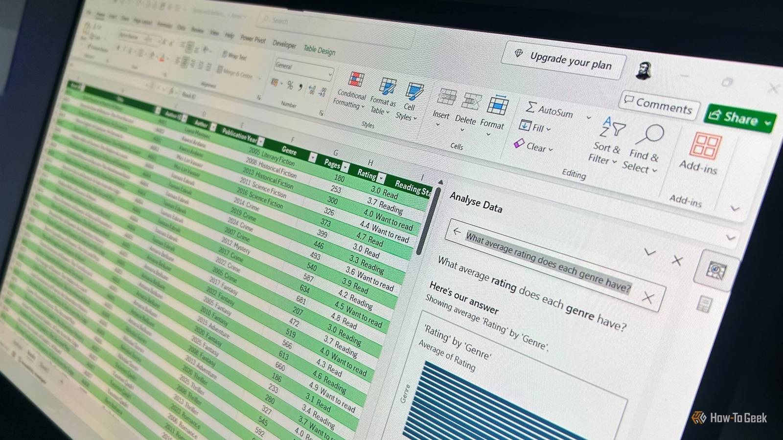
Analyze Data (previously called Ideas) can give you a useful starting point much faster.If you're using Excel for Microsoft 365 and have an internet connection, you can use this tool to automatically examine a structured dataset for patterns and summaries.To use it, select a single cell inside your data, then click Analyze Data in the Data tab.
In some versions of Excel, this button is found in the Home tab.Excel opens a pane containing automatically generated insight cards based on the information it finds.Close You can also type a question into the box at the top of the pane.
For example, because this dataset contains "Genre" and "Rating" columns, you could ask, "What average rating does each genre have?" Excel analyzes the data and produces a result that may include a summary table or visualization.If the result is useful, click the contextual Insert button to add the generated chart, PivotTable, or PivotChart to your worksheet.You can also try one of the suggested questions Excel generates based on your data.
Close Analyze Data works best when the source is properly structured.Make sure your data has a single header row and avoid unnecessary blank rows or columns.Formatting the range as an Excel table with Ctrl+T is also a good idea.
There's always more to discover in Excel This weekend is as good as any to explore some of Excel's lesser-known features.Custom Lists can make Excel follow your preferred order, Camera can keep a live view of important cells elsewhere in a workbook, and Analyze Data can quickly uncover patterns in a table.There's so much hidden away in Excel that the discovery never really ends.
So, if you still have some time to explore, take a look at some little-known Excel clicks that can further power up your spreadsheet skills.
Read More